Priors for symbolic regression

Download paper here

Abstract

When choosing between competing symbolic models for a data set, a human will naturally prefer the “simpler” expression or the one which more closely resembles equations previously seen in a similar context. This suggests a non-uniform prior on functions, which is, however, rarely considered within a symbolic regression (SR) framework. In this paper we develop methods to incorporate detailed prior information on both functions and their parameters into SR. Our prior on the structure of a function is based on a $n$-gram language model, which is sensitive to the arrangement of operators relative to one another in addition to the frequency of occurrence of each operator. We also develop a formalism based on the Fractional Bayes Factor to treat numerical parameter priors in such a way that models may be fairly compared though the Bayesian evidence, and explicitly compare Bayesian, Minimum Description Length and heuristic methods for model selection. We demonstrate the performance of our priors relative to literature standards on benchmarks and a real-world dataset from the field of cosmology.

Code

katz is publicly available

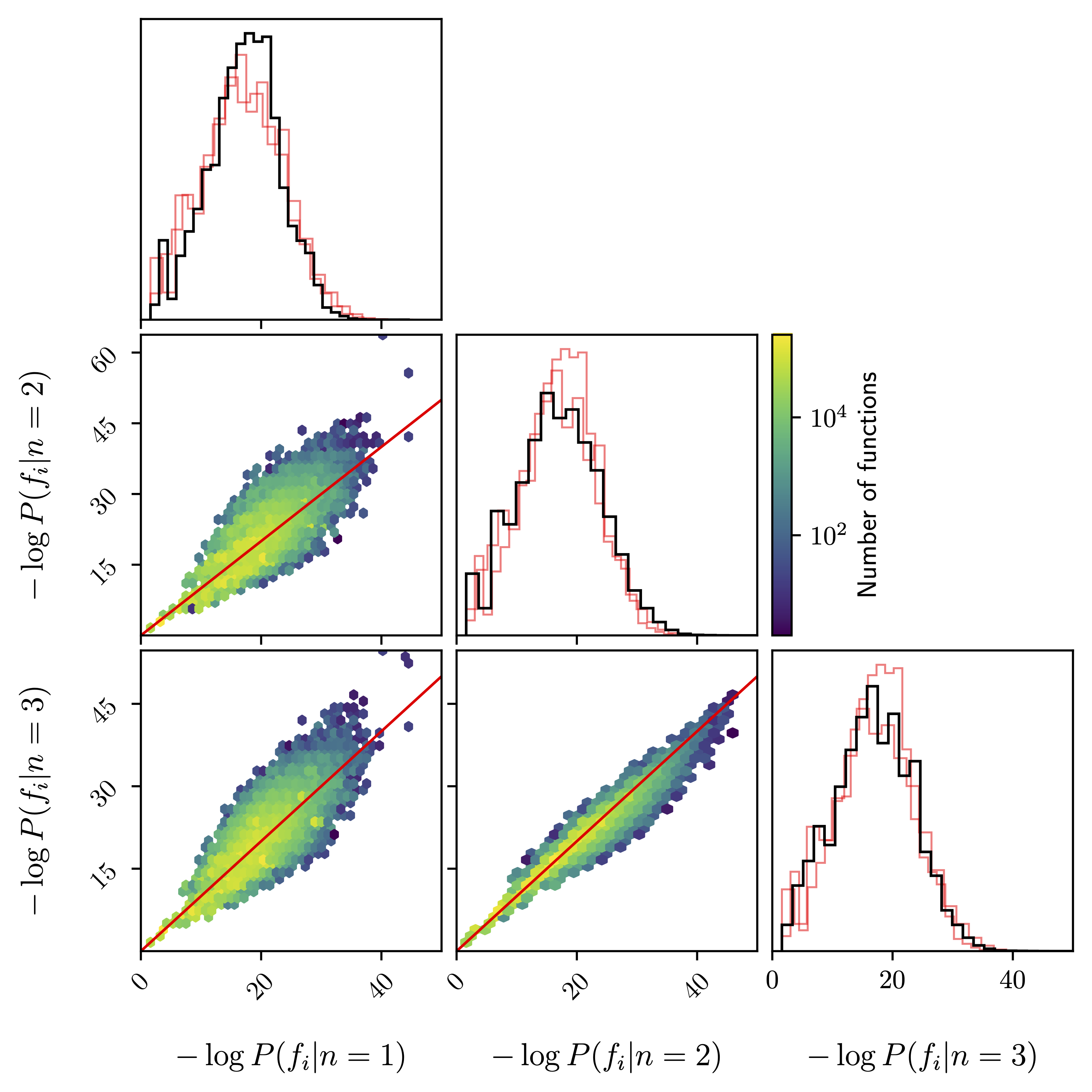One- and two-dimensional histograms of prior probabilities for all functions up to complexity 10 using the basis {$x$, $a$, ${\rm inv}$, $+$, $-$, $\times$, $\div$, ${\rm pow}$}. The priors are based on the compilation of scientific equations described in Section 2.4.2. and are evaluated using a back-off model with different lengths, $1\le n\le 3$. For the two-dimensional plots, points lying on the red line have an equal prior for both values of $n$ in the corresponding panel. In the one-dimensional plots, the black lines are the distributions for the corresponding $n$ and we plot the histograms for the other values of $n$ in red for reference.